Why XGBoost’s Gradients Aren’t the Same as Neural Networks

This article explains the fundamental differences between how gradients are utilized in XGBoost compared to neural networks. While neural networks use gradient descent to continuously fine-tune internal weights, XGBoost applies gradients directly to the predictions to see how much the model is missing the mark. Instead of tweaking existing parameters, it highlights how XGBoost uses these calculation errors to stack entirely new decision trees that step-by-step correct previous mistakes. Ultimately, the piece clarifies that neural networks optimize within a "weight space," whereas gradient boosting models optimize within a "prediction or function space."

When you hear “XGBoost uses gradients”, it’s natural to think of neural networks. After all, neural nets also use gradients to minimize loss.

But here’s the twist: the gradients in XGBoost mean something very different. Let’s break it down simply.

If you’re not familiar with ensemble models, check this out first to get a high-level understanding.

What is Ensemble Learning ? 😮

Now, let’s get back to our main topic: the comparison in really simple five steps.

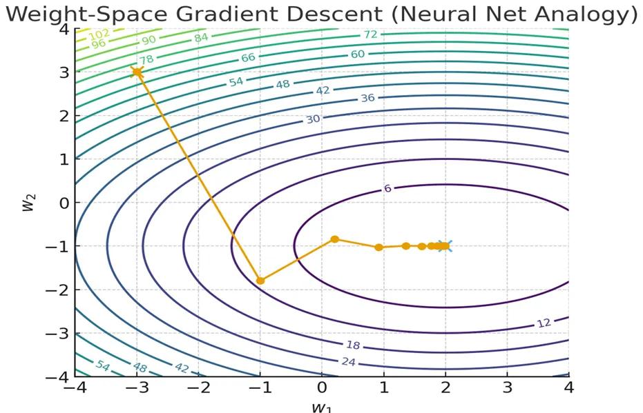
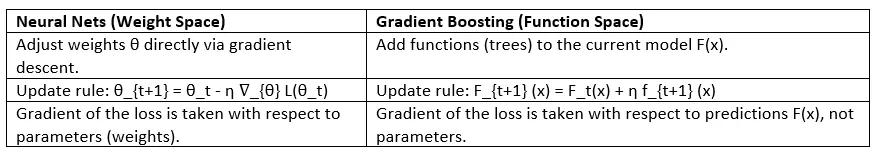
1. Neural Networks: Moving Weights Around

Imagine you’re standing on a mountain slope (the loss surface). Your goal is to walk downhill to reach the bottom.

In a neural net, the “position” is your weights (θ).
The gradient tells you which way is downhill in weight space.
Each step updates the weights:

\theta_{t+1} = \theta_t - \eta \nabla_{\theta} L(\theta_t)

Update Rule for Gradient Descent

Neural nets are like hikers adjusting their footsteps (weights) to get closer to the valley.

In neural networks, training means adjusting weights. This illustration shows gradient descent in weight space: starting from an initial point, the weights are updated step by step along the steepest descent path until they reach the minimum of the loss surface

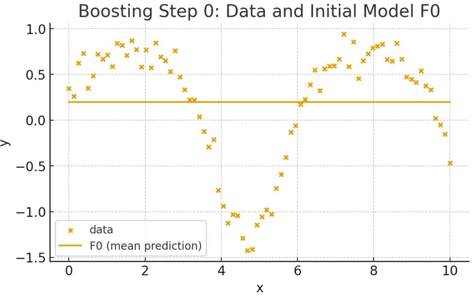
Author’s Construct Image — Author’s Construct

2. Gradient Boosting: Adding New Functions

Now imagine a different strategy. Instead of moving your feet, you call in new helpers. Each helper carries a little piece of wood to build a bridge that brings you closer to the valley.

In XGBoost, the “helpers” are new trees.
The model is an ensemble of all the trees so far:

F_t(x) = \sum_{k=1}^{t} f_k(x)

Compact Format of the Boosting Algorithm

At each step, we don’t move weights. We add a new function to improve predictions:

F_{t+1}(x) = F_t(x) + \eta f_{t+1}(x)

Update Rule for Gradient Boosting

The model starts with a simple baseline prediction, usually the mean of the target values. This gives us a flat line that clearly misses the patterns in the data.

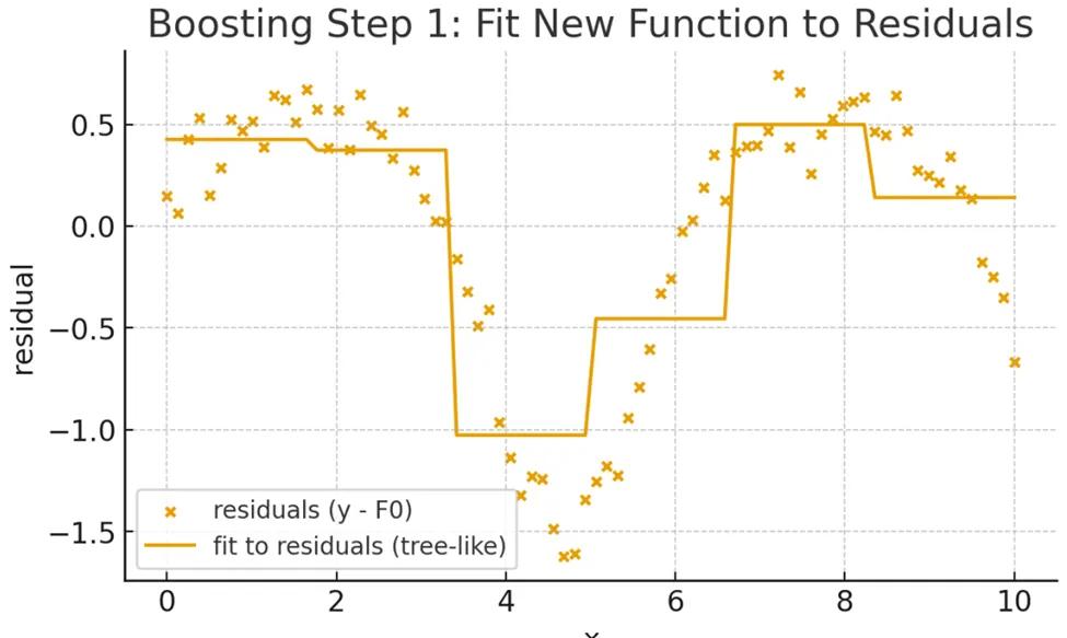
Baseline Model (F₀) Image — Baseline Model (F₀)

Then, we calculate the residuals (errors) between the baseline model and the actual data. A new weak learner (a shallow tree) is trained to fit these residuals, effectively learning how to correct the mistakes of the baseline.

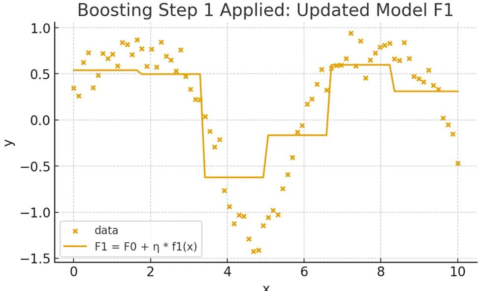
Residuals and New Tree (f₁(x)) Image — Residuals and New Tree (f₁(x))

We update the model by adding the new tree to the baseline. The combined model (F₁) now fits the data better than the flat baseline, capturing more structure.

Updated Model (F₁) Image — Updated Model (F₁)

3. So Where Do Gradients Come In?

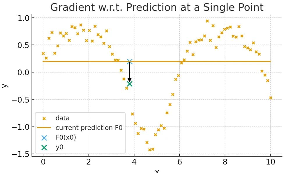
Here’s the trick: boosting still uses gradients, but not with respect to weights. Instead, it looks at how the loss changes with respect to the predictions.

For the general point (x_i, y_i)

g_i = \frac{\partial l(y_i, F_t(x_i))}{\partial F_t(x_i)}, \quad h_i = \frac{\partial^2 l(y_i, F_t(x_i))}{\partial F_t(x_i)^2}

First- and Second-Order Gradients in XGBoost

These tell us: “If I push the prediction up or down, how does the loss change?”

The next tree is trained to follow those gradients, effectively pointing in the steepest descent direction, but in prediction space, not weight space.

Gradient with Respect to Prediction at a Single Point Image — Gradient with Respect to Prediction at a Single Point

4. Understanding gᵢ and hᵢ

First-order gradient (gᵢ): how wrong we are at that point (residual).
Second-order gradient (hᵢ): how confident we are about the adjustment (curvature).
XGBoost combines them for more precise updates:

w^* = -\frac{\sum_{i} g_i}{\sum_{i} h_i + \lambda}

Optimal Leaf Weight Formula in XGBoost

Note: XGBoost assigns a weight to each leaf using both the first-order gradients g_i and the second-order gradients h_i.

This formula computes the optimal leaf value, balancing the gradient information with regularization λ.

In Simple this says:

g_i = “how wrong we are.”

h_i = “how confident we are about fixing it.”

5. Why It Matters

Neural Nets: You’re tuning weights. Hyperparameters like learning rate, batch size, initialization matter most.
XGBoost: You’re adding trees. Hyperparameters like depth, number of estimators, and regularization matter most.

Comparison of Weight-Space Gradient Descent (Neural Networks) and Function-Space Gradient Descent (Gradient Boosting) Image — Comparison of Weight-Space Gradient Descent (Neural Networks) and Function-Space Gradient Descent (Gradient Boosting)

In the end, both neural networks and gradient boosting rely on gradients, but they optimize in very different spaces. Neural nets move their weights step by step, like a hiker carefully marching downhill. Boosting, on the other hand, builds its path by stacking functions, each new tree nudging the model closer to the valley.

So, the next time you hear ‘XGBoost uses gradients’, don’t get confused like I did 😉, you might even feel like writing your own article about it.

Cheers to lifelong learners!!!